Happy GIS Day! More information about GIS Day can be found at http://www.gisday.com/ and some great videos about geospatial technologies at http://geospatialrevolution.psu.edu/
Tag Archives: GIS
Using GIS to determine stream sinuosity
Sinuosity is a measure of how much a river (or other linear feature) deviates from being straight. A truly straight river or road has a sinuosity of 1; as the number of meanders increases, sinuosity approaches 0.
I wrote a document describing how to determine the sinuosity of linear features years ago. I will update it for ArcGIS 10 as time permits, but the original document, written for ArcView 3.x and ArcGIS 8x/9x is available here.
Importing x,y data into ArcGIS
Importing a set of x,y coordinate pairs into ArcGIS is very straightforward, and can be a useful skill if you need to bring in simple coordinate data that is not already in a spatial format.
1) Acquire some data you want to display on a map. The source doesn’t matter: it might be locations recorded on a GPS unit that you don’t have a data cable for, coordinates determined from a topographic map, or a simple data set found on the internet. If you want your locations to integrate correctly with other layers (always a good thing in GIS) you will need to know both the coordinate system and datum used by the source data, e.g. latitude / longitude and NAD27.
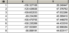
2) Format your data properly. This may be done in a spreadsheet program such as Google Spreadsheets <spreadsheets.google.com>, or the more ubiquitous Excel. To import properly into ArcGIS, your data file will require a minimum of three fields: a unique identifier for each data point, and the X (easting) and Y (northing) for each location. Other attribute data, if available, may go into additional columns, but your points will import fine with just these three pieces of information. Your file should also contain a header line that describes each field. It might be as simple as ID, X_coord, Y_coord. Additional fields are OK, but descriptions in each header are limited to seven characters and cannot have special characters or spaces. If you need spacing for readability, use underscores.

Be sure if you are using latitude/longitude coordinates that your northings are positive if north of the equator and eastings are negative if you are in the western hemisphere. Example: the coordinates for a location in Houghton, Michigan are -88.54820, 47.11535 in latitude/longitude and 382552, 5219145 in UTM zone 16, NAD 1983 datum. Omitting the “-” sign will put your points on the wrong side of the globe.
If your coordinates are in latitude/longitude, they should be in decimal degrees (DD) format before importing into ArcGIS. Locations in degrees, minutes and seconds (DMS) or decimal minutes (DM) format should first be converted to DD. There are converters available on the internet, but it is probably quicker to use Excel to perform the conversion.
D = Degrees M = Minutes S = Seconds .m = Decimal Minutes .s = Decimal Seconds
DM.m = Degrees, Minutes, Decimal Minutes (eg. 45°22.6333)
D.d = Degrees, Decimal Degrees (eg. 45.3772°)
DMS = Degrees, Minutes, Seconds (eg. 45°22’38”)
DMS –> DM.m (45°22’38” –> 45°22.6333)
◦ Divide S by 60 to get .m (38/60=.6333)
◦ Add .m to M to get M.m (22+.6333=22.6333)
DM.m –> D.d (45° 22.6333 –> 45.3772)
◦ Divide M.m by 60 to get .d (22.6333/60=.3772)
◦ Add .d to D to get D.d (45+.3772=45.3772)
D.d –> DM.m (45.3772 –> 45°22.6333
◦ Multiply .d by 60 to get M.m (.3772*60=22.6333)
DM.m –> DMS (45°22.6333 –> 45°22’38”)
◦ Multiply .m by 60 to get S(.6333*60=38)
DMS–>DD
◦ D + M/60 + S/3600 = DD
3) Save/export your data as a comma-delimited text file (CSV format in Google Spreadsheets or Excel). You may want to save a copy in native format (.xls in both Google spreadsheets and Excel) before exporting to .csv.
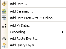
4) Add your .csv file to ArcMap by using the Add data tool (either by expanding the submenu under File> Add Data)  or by clicking the Add Data tool on the Standard toolbar
 ![]()
5) Right-click on your new layer and choose Display XY Data… Ensure that the X and Y fields were selected correctly by ArcMap – they should be right if you chose names that reflect the coordinate positions (northing and easting or x and y). Click the Edit… button, then Select… to select the coordinate system for your points, Add… and OK (3x). The correct coordinate system to use may be obtained from your GPS unit (under map setup or units); from the marginal information on your topo map; or from the metadata file that came with internet data. Look in geographic coordinate systems for latitude/longitude projection files, or in projected coordinate systems > UTM for UTM data.
Some possible suggestions:
- Coordinate Systems > Geographic Coordinate Systems > World > WGS1984.prj (default GPS datum)
- Coordinate Systems > Geographic Coordinate Systems > North America > NAD1983.prj (current North American datum)
- Coordinate Systems > Projected Coordinate Systems > UTM > NAD1983 > NAD 1983 UTM Zone 16N.prj (appropriate for most of the U.P.)
- Coordinate Systems > Projected Coordinate Systems > State Systems > NAD 1983 Michigan GeoRef (Meters).prj (projection and datum used by the State of Michigan)
6) You should now have a point layer at the top of your Table of Contents with the same name as your .csv file and the word Events on the end of the name.
This is an “event theme” and is a temporary layer. If you want a more permanent copy, right-click on the layer and choose Data > Export Data… Pick an output location—a geodatabase feature class or a directory for a shapefile—and enter a file name. Please change the name to something other than the default Export_Output – I suggest one that more accurately reflects the contents of the data layer. Click OK.
You now have a permanent layer, either a geodatabase feature class or shapefile, of your original ASCII (text) coordinates.
Assessing foodsheds in ArcGIS
From the latest ArcUser magazine: using ArcGIS to assess the path taken by food from its source to consumers in Chicago. Read the online article or a PDF
Color selection help
Color selection for maps can be a time-consuming activity. Computer monitors use additive colors (combinations of red, green, and blue) to create different shades, and monitors are backlit, using transmitted light to convey colors to the viewer. Printed maps, on the other hand, use subtractive colors (most often cyan, magenta, yellow, and black inks) to remove portions of white light reflected back to the viewer.
The main effect of these differing methods for producing colors is that hues you select on the monitor often look very different when printed out in hardcopy. This problem is compounded when different computer monitors or printers are used, as colors you were happy with can change dramatically when viewed or printed on different hardware.
Fortunately, a tool exists to help with choosing a set of colors for a map. ColorBrewer was developed by Cindy Brewer and Mark Harrower of Pennsylvania State University. It is an interactive, web-based tool that allows the user to 1) select the number of color classes needed, and 2) choose color schemes appropriate for numeric data (sequential schemes), numeric data with positive and negative values (diverging schemes with a neutral color in the center and darker colors at the extremes), or nominal data (qualitative schemes).
The color schemes in ColorBrewer were tested with subjects with color-impaired vision. You can choose to use only “color blind safe” colors, as well as “print friendly” and “photocopy-able” colors, though these choices limit the number of color schemes available. The best reason to use ColorBrewer, however, is the colors it provides are easily distinguished from each other.
ColorBrewer provides color information usable in several different coding systems (RGB, CMYK, and Hexadecimal) so it is useful for more than just colors for maps in a GIS. The values for your ColorBrewer color schemes can be exported to an Excel spreadsheet, and there is a plug-in tool for ArcGIS available. It is very user-friendly, but has excellent online help if you need it. Check it out!
Citing geospatial data
A common question that arises when writing a paper, thesis, or dissertation, is “How do I cite maps or spatial data”? I have cobbled together some examples over the years, found at various locations on the web, into a web page. Some of the source sites are no longer available (except perhaps at the Internet Wayback Machine), but the sources are still listed on the web page below.
A number of examples were drawn from: Cartographic Citations: A Style Guide, MAGERT Circular No. 1. Chicago: American Library Association, 1992. Thanks to the original authors of this publication.
See this page for my list of geospatial citation examples. I will update these examples as time permits.
How to generate random points in ArcGIS
One common activity in the natural resources field is the assessment of resources, such as vegetation, wildlife, or soil, in an area. There are several strategies available to perform these assessments. One method is to generate a number of random points in a given parcel of land where sampling will occur.
ArcGIS can generate a specified number of randomly-placed points within the boundary of a layer or inside a selected feature in a layer. The tool used to generate random points is found in Arc Toolbox : Data Management Tools > Feature Class > Create Random Points.
A one-page tutorial on generating random points is available here, or see below. It applies to ArcGIS 9.x and 10.
Generating Random Points in ArcGIS
A) Prepare a map document in ArcMap. Add any layers you need, including a polygon layer in which you would like to generate random points (e.g., stand boundaries). If necessary, select the polygon in which you would like the points contained. Verify that the data frame has the correct coordinate system defined.
B) Open ArcToolbox and open the Data Management Tools > Feature Class > Create random points tool.
C) Choose an output directory and a file name (random_points is suggested). If you have a constraining layer (a forest stand boundary or ownership boundary) select it. Enter the number of random points you need. Finally, if you need the points to be a minimum distance apart from one another, enter this value (E) and click OK. The points will be created and added to your map.
D) If you later need to identify your random points (which is likely), open the attribute table,
right-click on the field heading CID and choose Field Calculator. Build an expression
[FID]+1 and click OK. Your points should now be numbered from 1 to N. To add the coordinates for each point to the attribute table, open ArcToolbox > Data Management
Tools > Features > Add XY Coordinates. Choose your random point shapefile and
click OK. The fields POINT_X and POINT_Y will be added to the attribute table.
