Using the buffer wizard in ArcGIS 10.x

A complete PDF version of this post is available here

The Buffer Wizard is a ‘hidden’ add-on to ArcGIS. It allows for additional control when creating buffers. Specifically, it makes creating ‘inside’ buffers easier than the standard buffer tool.

The wizard was removed from the standard ArcMap user interface after ArcGIS 8.3, but is still available if you customize the user interface. I covered adding the buffer wizard in an earlier post (https://www.gis.mtu.edu/?p=448), but a quick summary of the steps is to open the Customize menu and choose Customize mode… Select the Commands tab, then enter the text ‘buffer wizard’ in the ‘Show commands containing’ box. Drag the tool to a toolbar (the Tools toolbar is suggested).

One possible application for this tool would be in preparation to perform sampling. You might want to assess the understory vegetation in a plot of land, but don’t want any of your sampling point to be within 10 meters of the edges of the plot.

1. Click the Buffer Wizard icon to start the tool

2. Choose the polygon layer that represents the area you want to sample from the drop-down list and click Next>.
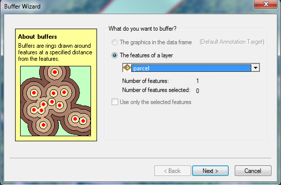
3. Specify your buffer distance (10) and verify the units are correct (meters). Note that you could choose to buffer based on an attribute table value or create multiple ring buffers here. Click Next>.
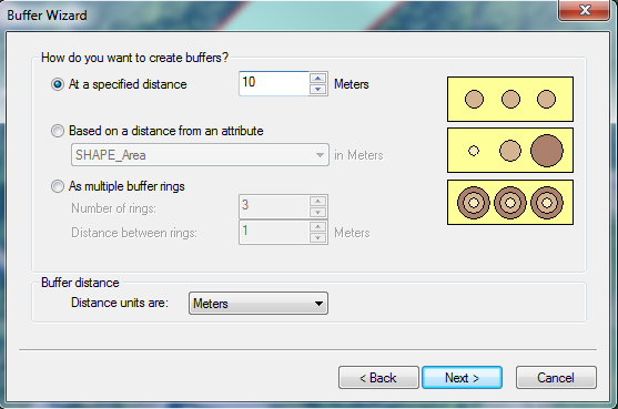
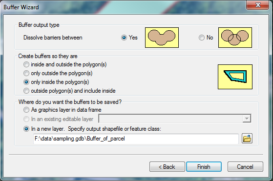
4. In the next window, select “only inside the polygons” and choose an output filename. This can be either a shapefile or a feature class in a geodatabase. Finish>.

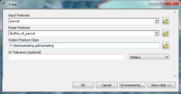
To remove areas within 10 meters of the boundary of your parcel, you will need to perform one additional step with the Erase tool. You can either use the Search tool (Windows > Search or Cmd-F) or expand ArcToolbox > Analysis Tools > Overlay > Erase. Your Input Features should be your Parcel layer, and the Erase Features your inside buffer. Choose an output file and click OK.

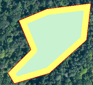
Here is how the original parcel appears, followed by the inside buffer and resulting polygon with the 10-meter border erased:
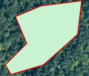


Original parcel (green with red border)
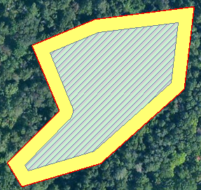

Inside buffer (yellow)


Final sampling area (crosshatched area)

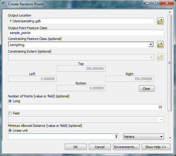
Now if you generate random sampling points using ArcToolbox > Data Management Tools > Feature Class > Create Random Points, you can use the final sampling area as a constraining feature class and ensure none of your points will be within 10 meters of the parcel boundary.
The resulting points are shown here:
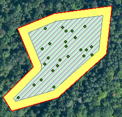
Note that none fall within the 10-meter buffer.

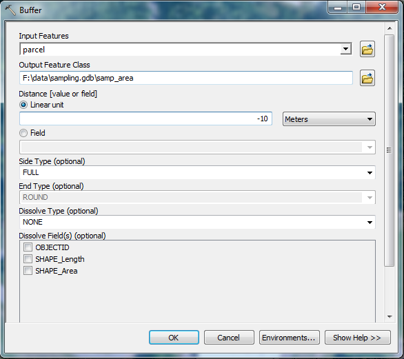
There is nearly always more than one way to accomplish a task in GIS. This workflow was written to illustrate the creation of an inside buffer using the Buffer Wizard, and a possible application with an inside buffer. The standard ArcGIS Buffer tool (ArcToolbox > Analysis Tools > Proximity > Buffer) lets you enter negative buffer distance values.

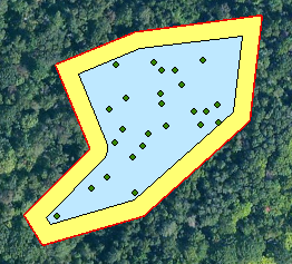
The resulting polygon has the same geometry as the original, just shrunk by the negative buffer amount (in the example above, 10 meters). It creates the same final polygon as the buffer inside then erase workflow above (buffer shown in blue below) with just a single step… You may have other needs for an inside buffer, though, so the Buffer Wizard can be quite useful.
ArcGIS ModelBuilder tutorial

I have written a short ModelBuilder tutorial that shown how to use an iterator to automate a repetitive process – converting a number of polygon feature classes to rasters in a geodatabase.

If you are interested in learning more about what can be done with the ModelBuilder, explore the ArcGIS Help files (search for ModelBuilder) and work through the two tutorials, or request a code to take the ModelBuilder course from the Virtual Campus.

Introduction to GIS course – first module

I am working on developing a series of self-paced GIS training modules. This first effort is designed for users who have never used ArcGIS before, and is a very simple introduction to using ArcMap.

The data are available to download here.

There is also a link to the data download in the exercise.

More updates and material to follow… You will need access to ArcMap 10.1 and have an Internet connection to complete this module.

ArcGIS for Desktop – “Tool not licensed” error

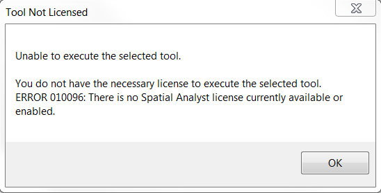
If you receive a ‘tool not licensed’ error when trying to use an ArcToolbox tool from an extension (Spatial Analyst, 3D Analyst, or others) then it’s likely you have not enabled the extension before trying to use it. If the extension has a toolbar, making it visible is not the same as enabling the extension.

Note that the error message states no… “license currently available or enabled“. The default install of ArcGIS includes all extensions, so it’s likely not enabled if you’re seeing this message.

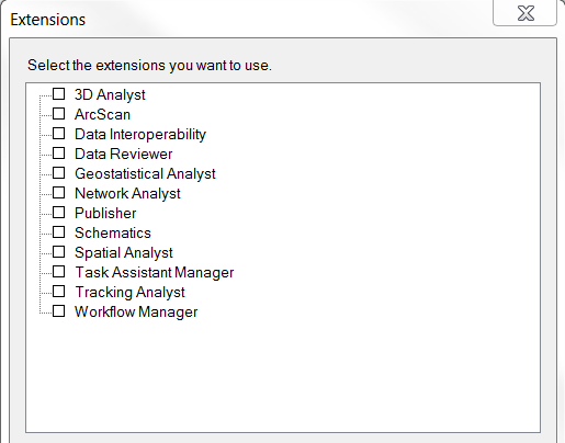
To remedy this, open the Customize menu and choose Extensions…

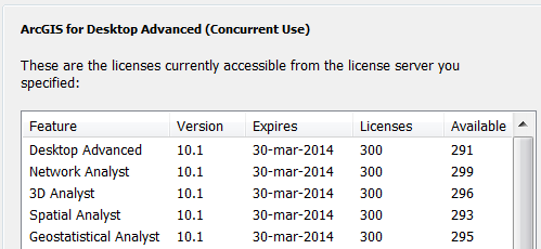
Check the box for any extension you wish to use, and click Close. Try re-running the tool and it should work. To verify if a license is available, open the ArcGIS Administrator and select the Availability panel. Extension licenses will be listed below ArcGIS…

How to update an ArcGIS student edition license

If you are running your own copy of ArcGIS – the Student Edition – the license is valid for one year. It is possible to renew your student license without re-installing ArcGIS or obtaining another install DVD. You will first need to get a new registration code. These are available by sending an email to it-help or to mdhyslop at mtu.edu

Detailed instructions for activating your license are available as a PDF: How to update an ArcGIS Student Edition license.

Please email mdhyslop with questions or comments.

How to determine the number of streams entering and exiting lakes using NHD data

Obtain data

Download a pre-staged file geodatabase for HUC subregion(s) of interest from http://nhd.usgs.gov/data.html and extract the contents of the download.

Prepare data

In ArcGIS, add the feature classes NHDWaterbodyNHDFlowline, and WBD\HU8 to your map. If you wish to work with lakes and ponds only, either perform a definition query on NHDWaterbodyto show only Type = Lake/pond (“FType” = 390) or select all FType = 390 and write the records out to a new feature class.

Remove the feature type “artificial path” from the feature class NHDFlowline. Artificial paths are created by NHD staff to simulate connections between inflows and outflows from water bodies (rivers entering and leaving lakes). Leaving these features in the data set will result in duplicate entries and an artificially (2x) high number of inflows and outflows. To remove these features from your analysis, you may either select all elements not flagged as ArtificialPath and write out to a new feature class, or perform a definition query to exclude them (“FType” <> 558).

You can create a new file geodatabase to hold your exported files and the results of your analysis or write the new data to the pre-staged geodatabase you downloaded above. Either option is fine.

Perform analysis

Intersect rivers and lakes

Open the Intersect (Analysis) tool and add your two layers (NDHFlowline and NHDWaterbody) as prepared above as Input Features. Change the Output Type (optional) from INPUT to POINT. This tool will create points wherever NHDFlowline features (rivers and streams) enter or exit lakes and ponds. Save your output file with a name that makes sense (e.g., include the HUC ID and InflowOutflow: NHD_403_InflowOutflow).

Add waterbody ID information to your point file

To obtain counts for each lake (total inflows and outflows) each lake will need a unique name. Unfortunately, many NHD lakes are unnamed and lake names are not unique (Examples? search for “Wolf Lake”, “Mud Lake”, or “Deer Lake” in any lakes database). Because of these ‘features’ of the data, generating a unique name isn’t as simple as it might be. A workable suggestion: add a new field to the lakes (NHDWaterbody) attribute table named UniqueName, type of Text and length of 50 characters. Ensure you have no records selected, and use the field calculator to populate the UniqueName field with the expression [GNIS_NAME] & “_’NHD’_” & [OBJECTID]  Replace ‘NHD‘ with the three-digit HUC prefix of the watershed you are working in (Lake Michigan is 403). The output will consist of something like “Wescott Lake_403_7” for records with a lake name, and “_403_17” for records where the lake was unnamed.

Next, perform a spatial join on your InflowOutflow points layer (created in the intersect step above). Right-click on this layer, and choose Joins and Relates > Join. Set the join type to “Join data from another layer based on spatial location” and choose your lakes layer (NHDWaterbody with the UniqueName field added) as the layer to join to your points. Under 2. in the Join Datawindow, set the relationship to is closest to it. (leaving the relationship set to the default it falls inside will result in no results (the points are not in the lakes, but on their borders). Name your output layer as something that makes sense (InflowOutflow_Lake_names) and save it in your file geodatabase.

Summarize results

Open the attribute table of your output file (InflowOutflow_Lake_Names). Find the UniqueName field and sort it (either ascending or descending) and look a the results. You should find multiple instances of many records (lakes with more than one inlet or outlet). All Distance values should be 0.

Right-click on the field UniqueName and choose Summarize. Choose the output destination (your file geodatabase unzipped or created above) and click OK. Answer Yes when prompted to add the summary table to the map. The resulting table will have one record for each lake (as found in UniqueName) and a Count_UniqueName value that summarizes the number of records of each UniqueName in your InflowOutflow_Lake_Names database. This Count value shows the number of streams entering or leaving each lake.

(Optional) Label lakes with Inflow / Outflow counts

As a last step you can join the summary table (created in the last step) to your lakes layer (NHDWaterbody) to label each lake with its total inflows and outflows. This join should be on the common field UniqueName. Be sure to Join attributes from a table, not Join data from another layer based on spatial location.