ArcGIS Pro crashing when editing symbology

This bug was introduced when Microsoft made some changes to their dotNet libraries back in November. The fix? Install a patch to the latest version of ArcGIS Pro 2.8 or 2.9. Links are below. You will need to be logged in to Google with your Michigan Tech credentials to download the patches.

Patch for ArcGIS Pro 2.8

Patch for ArcGIS Pro 2.9

ArcGIS Pro version 3.0 and up is not affected by this bug as it uses a newer version of dotNet…

Watershed modeling (Flow Direction) in ArcGIS Pro

You may run into issues when trying to run the Flow Direction tool in recent versions of ArcGIS Pro. This usually is evident as the tool taking an unusually long (infinite) amount of time to run to completion. A workaround that we have identified is as follows:

Make your selections as you normally would in the tool under the Parameters tab.

Next, switch to the Environments tab in the Flow Direction tool. Enter 0 under the Parallel Processing Factor option.

Click Run. The tool should run in a normal amount of time.

How to use ArcMap to create Garmin custom maps

ArcGIS includes a Map to KML tool that will create a KML file from an existing map document. The exported KMZ file will open in GoogleEarth or other KML file viewers, but the default image format it creates is not compatible with Garmin GPS units.

This video illustrates the export process, plus some quick edits you can make to create a Garmin-compatible KML file that will work on most recent map-enabled Garmin GPS units, such as the Dakota, Oregon, Colorado, Map78, map 62, and the eTrex 20 & 30. In addition to ArcMap, you should also have access to a text editor such as Notepad, an image editor such as the GIMP or ImageJ, and Google Earth.

To view your exported map on your Garmin GPS, you will need to ensure custom maps are enabled (they are by default). This process will vary slightly depending on the unit you have; it should be similar to the following (steps from a GPSMap 78):
MENU > Setup > Map > Map information / Select Map and scroll to Custom Maps. If Enabled – Custom Maps is shown, you should be all set. If Disabled – Custom Maps is shown, press ENTER, select Enable, and press ENTER again to toggle the setting. Press QUIT several times to exit Setup and select the map screen.

You should now be able to pan to the location for your map and view it on the GPS screen. You may need to zoom in to have the map appear.

If you are a QGIS user, open Plugins > Manage and Install Plugins… and search for GarminCustomMap. This plugin will export the current map canvas to a Garmin-compatible KMZ file.

*Update 6/20/2016

An ArcGIS tool has been developed to create Garmin custom maps directly. Details may be found at https://bitbucket.org/wankoelias/maptogarmincustommap/src 

Workflow outline for ArcGIS

  1. Set up map with layers symbolized as you like them; save MXD
  2. Create separate layer to denote map export extent
  3. Run Map to KML tool. Be sure to set Extent Properties to use the layer from 2. and the Data Content Properties to create a single composite image
  4. Use 7zip to extract the contents of the resulting KMZ file to a folder
  5. Convert the Composite.png PNG image to a JPG. Delete the original PNG
  6. Edit the doc.kml file by dropping it on a Notepad window. Change the extension on Composite.png to Composite.jpg and save the file and quit Notepad
  7. Select the two files (Composite.png and Doc.kml), right-click, and save to a new zip file
  8. Change the file extension from .zip to .kmz
  9. Copy the kmz file to your GPS unit > Garmin > CustomMaps folder
  10. If you don’t see your map, ensure your unit is configured to display custom maps

Generating a regular sampling grid in ArcGIS – an ArcToolbox tool

I have taken a workflow I developed a few years back and converted it to an ArcToolbox Tool (and ModelBuilder model). This tool should work for any license level of ArcGIS (Basic, Standard, Advanced). I developed the tool using ArcGIS 10.2.2, but saved versions for ArcGIS 9.3, 10.0 and 10.1 and later.

The tool has documentation (help) embedded, as well as metadata (item description) text. Be sure to set your Current and Scratch Workspace Environment settings under Geoprocessing > Environments… before trying to use the tool.

Here are links to download various versions of the tool These are shared from Google Drive, so look for the download link near the top of your browser window after clicking on one of the links below.

ArcGIS 9.3 Version
ArcGIS 10.0 Version
10.1 and later Version

Feedback (positive or constructive criticism) on this tool will be appreciated.

Finding and displaying color infrared imagery for the U.S.

I. Finding and downloading (recent) CIR imagery

If you need color infrared (false-color) photos for vegetation analysis, you may find these instructions useful. Many sites (e.g., the USDA Geo Gateway) strip the near-IR band from recent imagery to keep file sizes small. Fortunately, the complete, four-band images are available from the National Map web site. Keep reading to learn how to find and use CIR imagery.

1) Go to http://nationalmap.gov/viewer.html

2) Click on or visit http://viewer.nationalmap.gov/viewer/

3) Zoom in on your area of interest using either the scroll wheel on your mouse or the zoom tool  at the top of the map window
4) Click the Download Data button  You will be asked if you wish to define a download area by drawing a box, by using 1:24k quad sheets, by using the entire visible map, or by entering coordinates. Choose the first option (bounding box). Click and drag over your area of interest (AOI).


5) Next, you are presented with list of available data for your AOI. Choose Orthoimagery and click Next.

6) You will be shown a list of imagery available for your AOI. The first option, 10:1 Compressed NAIP,  contains the 2010-2012 4-band imagery. (Note under “Band” these data are listed as 4B (red, green, blue, and near-infrared)). Check the box next to 10:1Compressed NAIP, then click Next.

7) Your ‘shopping cart’ will appear on the left side of your browser window. Click the Checkout button.

8) Enter your email address twice on the next screen and click Place Order.

9) You should see a confirmation of your order in a pop-up window. Click OK to dismiss the pop-up.

You will receive an e-mail message with links to your download. Note that orthophotos are distributed in 3.75-minute tiles, so each 7.5-minute (1:24,000 scale USGS quagrangle map) will be covered by four photos. A county may require several dozen images for complete coverage.

Four USGS 7.5-minute quads are shown in the image above (Point Nipigon, Cheboygan, Aloha, and Mullett Lake). Sixteen images would need to be downloaded to cover this ~18 x ~12-mile area.


II. Displaying Color infrared (CIR) Imagery in ArcGIS

1) After downloading your images, start ArcMap and open a new map document.

2) Use the ArcCatalog tab or the Add Data tool to browse to your data folder. Add the downloaded images to your map. By default, ArcGIS will display the images using a standard, “visible color” scheme (red-green-blue).

3) Right-click on an image and choose Properties… 

4) Choose the Symbology tab and change Red to Band_4, Green to Band_1, and Blue to Band_2. Click Apply, then OK.

5) Your image should change from primarily green to red (assuming you are viewing a forested or otherwise vegetated area).

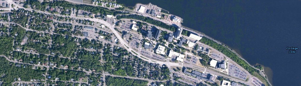
The top image above is shown in standard (R-G-B) colors; the one below in ‘false color’ NIR-R-G. Healthy, chlorophyll-rich green vegetation is depicted in reds and pinks in false color imagery. Note that Sherman Field, Michigan Tech’s football field, is artificial turf: it appears green to the naked eye (standard color image), but is nearly black on the CIR image. Infrared film was originally known as ‘camouflage detection film’ due to the ability to resolve ‘fake’ vegetation in this manner.

6) Repeat the band settings (changing to bands 4-1-2) for each image in your map.


III. Displaying Color Infrared (CIR) Imagery in QGIS

1) After downloading your images, start QGIS and open a new project document (loading a new, empty project document is the default behavior).

2) Use the Browser to view your data folder. If you don’t see the Browser, go to View > Panels and ensure that Browser is checked.


3) Next, expand the directory that contains the images you downloaded. Add any images you need by dragging them from the Browser to the map. By default, QGIS will display color imagery  using a standard, “visible color” scheme (red-green-blue).

You could instead use the Add Raster Layer tool (above) to add your images but I find the Browser easier to use.

4) Right-click on an image in your Layers list and choose Properties 

5) Select the Style panel. Set the Red band to display Band 4, the Green to Band 1, and the Blue to Band 2. Click Apply and then OK.

6) QGIS will now display your image in shades of red instead of green (assuming you are viewing a forested or otherwise vegetated area).

Note that conifers have different leaf cell structure and contain less chlorophyll than deciduous vegetation, so along with differences in texture (conifers often appear coarser), coniferous trees are usually darker on false-color imagery because they reflect less energy in the NIR band. A coniferous stand is highlighted in the two images above.

Calculating stream sinuosity (in esri products)

A river’s sinuosity is its tendency to meander back and forth across its floodplain, in an S-shaped pattern, over time. As the stream moves across the landscape, it may leave behind evidence of where the river channel once was (these can take the form of meander scars or oxbow lakes). These patterns usually appear in stream channels found in softer sediments. If a river’s course is bedrock-controlled, other factors—primarily rock strength and structure—control the river’s flow. Few stream courses are completely straight, and most exhibit meanders.

If you ever work with hydrologic data in GIS, you may wish to determine the sinuosity for an entire river or a particular ‘reach‘ of a river of interest. A stream that doesn’t meander at all has a sinuosity of 1. The more meanders in a stream, the closer the sinuosity value will get to 0. Fortunately, it’s simple to determine the sinuosity of a line using either the field calculator or Python. Depending on the version of GIS software you are using, the method differs. See this post for details for ArcView 3 (old!) and ArcMap 8.x-10.2.

Citing maps and data

A Twitter conversation this week reminded me that it’s not always easy to cite data or maps you may use in your reports, papers, or theses. As a result, I revisited and updated a web resource I put together 10 or more years ago that lists sample citations for GIS maps and data, and points to other web resources with formatting guides: Citing Geospatial Data Remember, you will need to choose a citation format acceptable to your instructor, advisor, or journal editor.